Introduction
The time variable, i.e. the length of time until an event occurs, is one of many different research variables that can be recorded and statistically analyzed. For example, in survival analysis, we are focused on patient’s survival, which is the main clinical interest, and death is the unwanted event. Any other event may also be taken as an endpoint as long as it can be described as binary, e.g. 1 if the event occurred and 0 if it did not occur (binary setting assumes that no other event is possible). For example, we can analyze time to graduation in a population of students and report a graduation rate at five years or determine a median graduation time. In biomedicine, there are many possible uses of this type of analysis, such as analyzing time to recovery after a therapeutic procedure, time to reach a predefined blood level of a substance, time to relapse of disease, time to hospital discharge, and many others.
Why do we need special methods to analyze survival data?
The main difficulty in the analysis of survival data is that patients are not enrolled in the study all at the same time, but dropwise (the follow-up of each patient starts at a different time point). For example, we cannot perform surgery on 50 patients at the same time in order to start observing their survival from that moment on. Patients with the disease of our interest come over time, one by one, not on the day set as the beginning of the study. Therefore, patients included in the survival analysis are, as a rule, followed up for different lengths of time due to their gradual influx (1). Patients enrolled later in the study are followed up for a shorter time and usually are still alive at the time of data analysis, while others drop out at some point during the study and are lost from observation (lost to follow-up). In either case, we cannot evaluate what happened to them after the time of last visit when they were still alive. Information on such patients remains unknown, i.e. censored, but we record their status as if they were still alive (by 0). If we analyzed such censored data using standard statistical methods, for example, if we compared the median time needed to reach the endpoint in two groups, we would receive misleading results (2).
If we were to calculate a 5-year survival rate for 50 patients who underwent a particular treatment, we would have to observe each one of these patients (even the ones who died) for five years and then divide the number of survivors by the total number of patients (Nsurviving/Ntotal) (3). Such an approach is usually called a direct method and, in the above example, it would take longer than five years to calculate the 5-year survival rate. All patients who were followed up for less than five years, whether alive or dead would have to be excluded from the calculation. This is a disadvantage of the direct method as it goes against the rule of intention-to-treat analysis. Another disadvantage of the direct method of calculation (3) is that we cannot calculate the mean survival time before we know all survival times (4) (e.g. until all patients die). In some cases, it could take decades. In the direct method, some of the censored surviving times would be discarded, although they contain valuable information about survival up to some point in time.
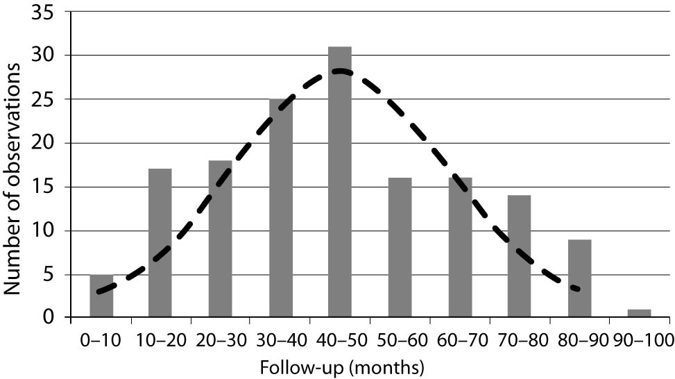
In a typical clinical study, patient follow-up times usually do not follow a normal distribution (Figure 1) and, therefore, follow-up data have to be presented as median with range and analyzed using nonparametric statistical methods.
Figure 1. Survival times usually do not have normal distribution. The histogram presents a follow-up (months) of 152 patients from the study (10). The normal distribution was calculated and is presented by a dashed line (empirical data were not compared using one-sample normality test).
About censoring
Whenever we analyze censored data, we have to ensure that the entry and censoring criteria remain the same during the entire enrollment period (5,6). In other words, we must strictly define the starting point (intended-to-treat or treated patients) and the endpoint (death, but also death only from a specific cause; disease relapse; etc.). We also have to recheck data on all patients lost to follow-up. The proportion of patients lost to follow-up should be the smallest possible, because too many patients lost from observation can make survival analysis unreliable. Removing or recording unfavorable outcomes as lost is not allowed, because it alters the results and leads to wrong conclusions.
Actuarial (life-table) method and Kaplan-Meier method
Insurance companies are always interested in how likely someone is to die/live for some defined period of time. For that purpose, they have developed a life-table method to calculate the data in certain groups of people. This method is also called the actuarial method (actuary – professional dealing with financial risks) (1). It divides the observation period into equal time intervals and calculates the proportion dying in each one of them. Proportion dying in each time interval is set as Ndied/Nexposed or Ndied/(Ntotal in interval - Ncencored/2). The method assumes that censored observations contribute only halfway to the number of patients currently at risk (during given time interval), and that is called actuarial assumption. Someone who lived up to the 8th time interval had to live through seven previous time intervals, so their risk of dying accumulates. It should be noted that proportions of dying and surviving add up to 1 (proportion dying = 1 – proportion surviving). A cumulative proportion dying is gradually increasing with each time interval, as it is multiplied with proportion dying in preceding time intervals, while a cumulative proportion surviving is decreasing and represents the survival rate up to the time interval. Life-table method is useful when death and censored observations are already organized in time intervals, which is rarely the case in biomedical research.
Kaplan-Meier method (product-limit method) (1,7,8) uses a similar principle to calculate the cumulative proportion surviving over time, with a new time interval starting with each new death. Censored observations are placed in corresponding intervals and contribute to the total number of subjects (if censored observation happens at the same time as death, it is assumed to happen a bit after and is placed in the following interval). To calculate proportion dying, the method simply divides the number of deaths in a time interval (always 1) with the total number of subjects at the beginning of the interval. Cumulative proportion dying and surviving are calculated in the same manner as in actuarial method. The first interval always ends with the first (earliest) death, does not include any death times, and has a surviving proportion of 100%.
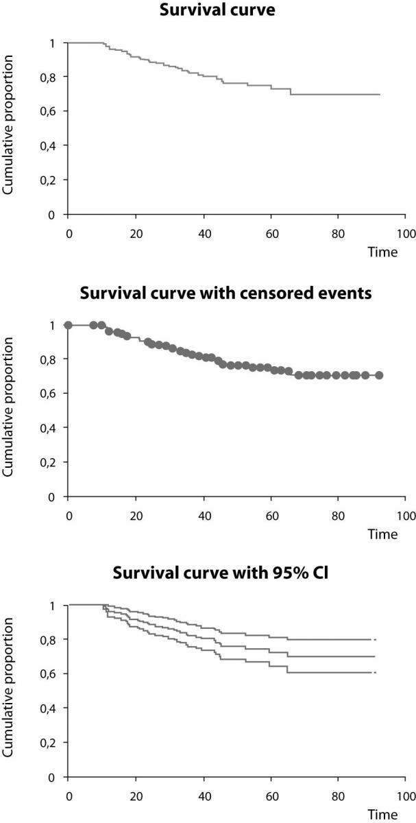
Proportions surviving through consecutive intervals may be presented as a survival curve, which represents a survival function over time (Figure 2). This plot is a step function with gradually falling steps if deaths in the following intervals occur. Survival rate (cumulative proportion surviving) can be read from the curve at any time point. Median survival time is the time point at which 50% of patients died/survived and can also be read from the survival curve (1,2,4,8). The last interval is always open and represents the survival rate from the last death observed (Kaplan-Meier method) or defined interval border (actuarial method) to infinity. The analysis of survival data by Kaplan-Meier, actuarial or direct method (in the last case, incomplete observations must be excluded) produces almost the same results, but Kaplan-Meier method is usually the method of choice as it produces the most accurate information for any given follow-up time. When there are no censored data, i.e., none of patients is lost and all observed patients died, the results of all three methods are the same (3).

Figure 2. Survival curves from the study (10) created using Kaplain-Meier estimation. The survival curve itself (upper), with designated censored events (middle), and survival curve with the upper and lower 95% confidence interval curves (lower). Time is shown in months.
Calculating survival using Excel sheets
For the didactic purposes of this text, we prepared a workbook for MS Excel program (ver. 2002, Microsoft, Redmond, Washington, USA), which is freely available as supplementary file at
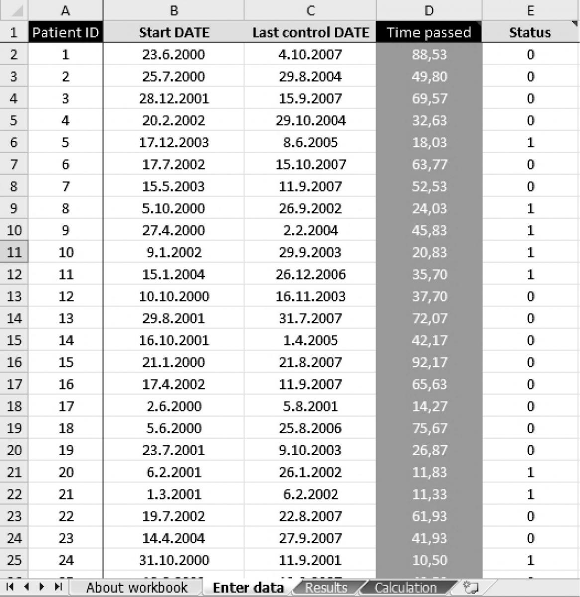
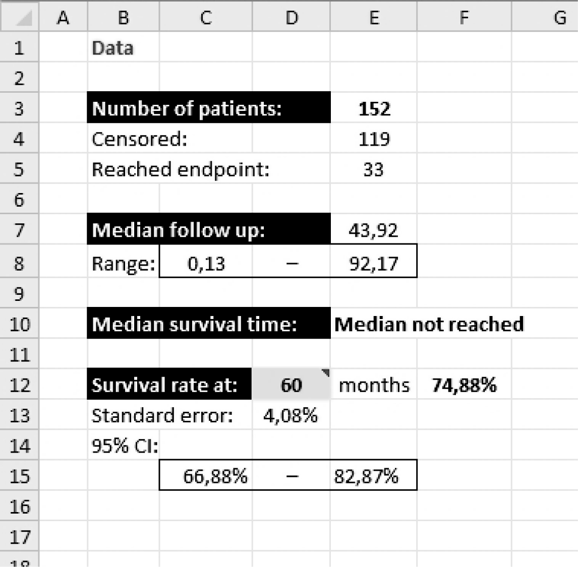
http://www.biochemia-medica.com. It is based on most commonly used Kaplan-Meier method and intended to help the reader understand how Kaplan-Meier method is conceptualized and how it may be used to obtain statistics and survival curves needed to describe a sample of patients. A reader can copy/paste his own recorded data into provided columns either as a start date, last control date and status indicator (1 – dead, 0 – alive), or directly as prerecorded follow-up time and status indicator (Figure 3). The program reports the total number of patients, number of patients reaching the endpoint, number of censored observations, and median follow-up time with range (from the smallest to the largest observed time) (Figure 4). The median survival time is reported only if it is reached. The survival rate can be calculated for any point in time by entering the desired time in a specified box (entry is preset to 60 months to obtain the usual 5-year survival rate). Survival rates are calculated with standard errors and provided with 95% confidence intervals. The survival curve and survival curve with 95% confidence interval are plotted (Figure 4).

Figure 3. Data from the entry page of the workbook. Each patient from the study (10) is designated with a serial identity number (ID, column A). Survival times were calculated from the start date (column B) and the date of last control (column C) for each patient (in months, column D) or were entered directly. Each patient is designated with a status indicator (column E: 0 – censored, 1 – dead).
Figure 4. Numerical results of survival data analysis from the workbook summarizing the number of patients from the study (10), median follow-up time with data range (in months, in this example), median survival time, and survival rate at 60 months with respective standard error and 95% confidence interval.
Comparing two survival curves
A number of factors can impact a survival rate over time and cause survival curve to change. We can test if some factor significantly changes the survival by comparing two groups using log-rank test. The test assumes no difference in dying proportions between two groups and calculates the proportion dying in every time interval (1,5). Then it multiplies this number with the current number at risk in each group to calculate the expected number of deaths. After summing up all expected deaths, we can compare the expected number of deaths with the observed number of deaths (for each group independently), usually using c2-test. There are different types of log-rank tests, some named after respective authors, that slightly differ in their calculations (Cox-Mantel, Peto, Mantel-Haenszel, and some others) (8). When test statistic is obtained, the P-value is read from the normal or c2-distribution for one degree of freedom (depending on the type of log-rank calculation used). The slope of survival curve at some point in time is termed hazard and represents the rate of dying for that follow-up time.
We can use log-rank test only if survival curves do not cross each other (the assumption of proportional hazards during the follow-up, i.e. the risk of event in group A is consistently greater or lower than risk in Group B). If this is true, the proportion can be calculated by comparing the expected and observed deaths in both groups. It is called hazard ratio and allows us to estimate the degree to which a tested factor contributes to survival. For example, if hazard ratio and lower limit of its 95% confidence interval are higher than 1, we can be 95% certain that this factor increases the risk of dying by the value of hazard ratio (9). In case survival curves cross later during follow up, special type of weighted log-rank test (Breslow-Gehan generalization of Wilcoxon test) can be used as it gives more weight to early observations when calculating test statistic. However, we can not use hazard ratio or make conclusions about difference in survival after point where curves cross each other.
Conclusion
When analyzing the time to the occurrence of an event, one has to be wary of falling into statistical traps. Special methods have been developed to summarize and compare this type of data without losing valuable information contained in censored observations. Kaplan-Meier method is most widely used for summarizing data. Variants of log-rank test are usually used for comparing two survival curves. These methods also provide an estimate of how much a tested factor increases the risk of dying, which is called hazard ratio.
Acknowledgments
All data presented in Figures 1-4 were original data on patients with oral cancer from Ivica Luksic’s Ph.D. dissertation (10) and were used here with author’s permission only for the presentation of statistical methodology. Authors would like to thank Dr Aleksandra Mišak for the editing of the manuscript.
Notes
Potential conflict of interest
None declared.
References
1. Collet D. Some non-parametric procedures. In: Modelling survival data in medical research. London: Chapman&Hall, 1994. p. 15-51.
2. Petrie A, Sabin C. Survival analysis. In: Medical statistics at glance. Carlton-Oxford: Blackwell Science, 2005. p. 119-21.
3. American Joint Committee on Cancer. Reporting of cancer survival and end results. Manual for staging of cancer. London – Sydney: J. B. Lippincott Co., 1988. p. 12-24.
4. Motulsky H. Survival curves. In: Intuitive biostatistics. New York: Oxford University Press, 1995. p. 53-9.
5. Motulsky H. Comparing two survival curves. In: Intuitive biostatistics. New York: Oxford University Press, 1995. p. 272-6.
6.Clark TG, Bradburn MJ, Love SB, Altman DG. Survival analysis part I: basic concepts and first analyses. Br J Cancer 2003;89:232-8.
7. Kaplan EL, Meier P. Nonparametric estimation from incomplete observations. J Am Stat Assoc 1958;53:457–81.
8. Dawson-Saunders B, Trapp RG. Analyzing research questions about survival. In: Basic&Clinical biostatistics. New York – Toronto: Lange Medical Books/McGraw-Hill; 2004. p. 221-44.
9. Simundic AM. Confidence interval. Biochem Med 2008;18: 154-61.
10. Luksic I. The significance of myofibrobastic proliferation in the extracellular matrix of oral cavity carcinoma on incidence of regional metastases. Ph.D (in Croatian). School of Dental Medicine, University of Zagreb; 2008.
